From dict to DashTable: How Dragonfly cuts memory overhead by 40%

Every Redis instance lives and dies by its dictionary. When you SET k v, Redis lands the key in a hash table called dict. When you run BGSAVE, that same dict is what gets serialized (via fork() — ouch! https://www.dragonflydb.io/blog/balanced-vs-unbalanced). When you run a server for months under write-heavy load, dict's memory overhead is one of the things slowly bleeding your cloud bill.

So when we built Dragonfly, we went looking for something lighter — lighter on memory overhead, lighter on resize latency, lighter on the process model. We found it in a data structure called DashTable, and understanding how it works explains a surprising number of Dragonfly's most distinctive properties: smaller memory footprint, no fork during saves, cheaper expiry. None of those are accidents. They all flow from the same design decisions baked into the data structure. And we know it works because we measured it. Full details and a ground-up walkthrough of DashTable below.

The Problem With Redis's Dictionary

Redis dict is a textbook separate-chaining hash table, and that shows in the memory numbers. The structure is two hash tables (ht[0] and  ht[1]), each implemented as a bucket array where every bucket holds a pointer to a linked list of dictEntry nodes. Before we get to DashTable, it's important to discuss the design costs.

Redis handles growth by allocating a second hash table ht[1] alongside the live ht[0] and migrating keys incrementally, a few buckets per operation, until ht[0] is empty. The goal is to tame P99 latency by avoiding large stalls of the entire system.

In practice; it trades one problem for three.

First, memory overhead spikes during rehash. When ht[0] is full and rehashing begins, ht[1] is allocated immediately at 2x the current capacity. Both tables coexist in memory until the migration completes.The spike:  ht[1] has capacity 2N. dictEntry pointer is 8bytes so 16N bytes landing on top of the 8N already paid for the ht[0] bucket array and the 24N for the dictEntry nodes. Total at peak: 48N, before a single key has moved. For a server holding billions of keys, that jump can be measured in dozens of gigabytes:

Second, rehash is slower than it looks. Every write operation on a rehashing dict includes a step that migrates one bucket from ht[0] to ht[1]. Every key read has to check both tables. The overhead is diffused rather than concentrated - spread across thousands of operations rather than one pause - but it is never zero. Under high write throughput, the migration can lag, keeping both tables live longer than intended and sustaining the memory overhead for extended periods. Pausing the server for large migrations is not an option and that’s why it is amortized (incrementally).

Third, the cycle repeats. Once ht[1] becomes the new ht[0] and the tables fill up the whole process restarts. Redis's growth policy means a server growing in key size will cycle through these rehash windows repeatedly over its lifetime. Table resizing is not a one time event.

None of this is a design flaw and it's a perfectly reasonable hash table from an era when these tradeoffs were standard.[^1]

The one idea behind DashTable: Segments as leafs

The algorithm underneath DashTable is called extendible hashing. It was invented by Fagin, Nievergelt, Pippenger, and Strong in 1979 and published in the Journal of the ACM. It spent the next four decades mostly in textbooks until it resurfaced in a 2020 VLDB paper (DASH: Scalable Hashing on Persistent Memory) that adapted and extended it for modern hardware. Dragonfly's implementation builds on that paper.

The core insight is a change in what the top-level array stores. 

In a classic hash table, the array holds pointers to the first node of a linked list. In extendible hashing, the array holds pointers to segments — fixed-size, self-contained mini-hash tables. Each segment is made of buckets, and each bucket contains a small fixed number of entry slots. A key’s hash first chooses a segment, then chooses a bucket inside that segment.

The top-level array is called the directory. The easiest way to understand the directory is as an array representation of a binary tree over hash prefixes.

The directory has a global depth. If the global depth is K, the directory has 2^K entries, and DashTable uses K bits from a key’s hash to choose one directory entry.

But not every directory entry points to a different segment. Multiple directory entries can point to the same segment.

That is where local depth comes in. A segment’s local depth says how many hash-prefix bits identify that segment.

In this diagram, the directory has global depth 2, so it has four entries: 00, 01, 10, and 11.

The important detail is Segment C. Both 10 and 11 point to the same segment. That means Segment C does not distinguish two hash bits yet. It only distinguishes the first bit, 1, so its local depth is 1.

In other words, Segment C owns the whole prefix range 1*:

10 —> Segment C

11 —> Segment C

In the full directory tree, 10 and 11 are two separate leaves. In the compressed segment tree, they are collapsed into one segment representing prefix 1*.

At this point, the important idea is simple: a directory can have many entries, but those entries do not necessarily point to distinct segments. A segment can represent an entire prefix range. Growth happens by splitting one of those ranges.

Growth means splitting one prefix

Eventually, an insertion may reach a segment where DashTable cannot place the new entry. That does not necessarily mean the segment is completely full. It means the insertion algorithm has exhausted the ways it is willing to place the entry inside that segment.

In a traditional hash table, this is where the table-level resize story begins: allocate a larger array and gradually move entries from the old table to the new one.

DashTable does something smaller.

Continuing from the diagram above, Segment C owns the prefix range 1*. Both directory entries 10 and 11 point to it:

10 —> Segment C

11 —> Segment C

Now suppose an insertion cannot be placed in Segment C. DashTable does not resize the whole table. It splits the prefix range owned by Segment C.

After the split, DashTable uses one more hash bit to divide 1* into two smaller ranges:

10 —> Segment C

11 —> Segment C'

DashTable allocates one new sibling segment, increases Segment C’s local depth from 1 to 2, and redistributes only the entries that were stored in Segment C.

Only Segment C is involved. Keys in Segment A, Segment B, and every other segment stay exactly where they are.

This is the central growth property of DashTable: a failed placement causes one prefix range to split, not the whole keyspace to migrate. The cost of growth is bounded by the size of one segment.

When the directory has to grow

The Segment C example showed the easy case: Segment C had local depth 1 while the directory had global depth 2. The directory already had separate entries for 10 and 11, so DashTable could split the segment by updating pointers.

But that is not always true.

A segment split creates two prefix ranges where there used to be one. The directory must be deep enough to point to both of them. If a segment’s local depth is smaller than the directory’s global depth, the directory already has enough entries to represent the split. DashTable only updates the relevant directory pointers.

If the segment’s local depth equals the global depth, the directory is not deep enough yet. DashTable first doubles the directory, increasing the global depth by one. Then it performs the segment split.

So the rule is:

local depth < global depth —> split the segment 

local depth == global depth -> grow the directory, then split the segment

The important part is that directory growth does not move key/value entries. It only expands the pointer structure so the new sibling segment can be addressed. The actual data movement still happens inside one segment.

To make this concrete, imagine a directory of global depth = 1:

It has two entries:

0 —> Segment A

1 —> Segment B

Suppose an insertion cannot be placed in Segment A. Segment A also has local depth 1, so its local depth equals the directory’s global depth. There is no deeper directory entry available to represent the split.

DashTable first doubles the directory:

00 —> Segment A

01 —> Segment A

10 —> Segment B

11 —> Segment B

Then it splits Segment A using one more hash bit:

00 —> Segment A

01 —> Segment A'

10 —> Segment B

11 —> Segment B

Notice that Segment B did not split. Both `10` and `11` still point to the same segment. The directory grew, but the only data movement happened inside Segment A.

How does Dragonfly finds space before splitting

The split described above is the fallback path, not the first thing Dragonfly tries.

In Dragonfly, a segment contains 56 regular buckets and 4 stash buckets. Each bucket has 14 slots, and each slot can hold one entry. So a segment can store up to 840 entries.

That fixed capacity is what makes the split cost bounded: when Dragonfly splits a segment, it only has to redistribute the entries inside that segment, not the whole table.

On insertion, Dragonfly first hashes the key to find the target segment and bucket. If the ideal bucket has room, the entry is inserted there. If not, Dragonfly tries several ways to find space inside the same segment before deciding to split.

At a high level, the insertion path is:

1. Try the target bucket.

2. Try nearby buckets.

3. Try to displace an existing entry.

4. Try the stash buckets.

5. If none of those work, split the segment.

A segment split does not necessarily mean the segment had zero empty capacity left. It means Dragonfly could not place this particular entry using its normal placement strategy.

Dragonfly also uses expiry information to avoid unnecessary splits. If a segment contains expired keys, Dragonfly can clean them up and reuse the freed space instead of allocating a sibling segment.

So the real goal of the insertion algorithm is simple: keep each segment highly utilized, and split only when local placement fails.

Why this makes the growth predictable

At this point, the contrast with Redis is the crucial part.

Redis grows a dictionary by maintaining two hash tables during rehash and gradually migrating buckets from the old table to the new one. The work is amortized, but the resize still involves the table as a whole.

DashTable grows locally.

A failed insertion affects one segment. The split redistributes entries from that segment only. If the directory has to grow, it grows by copying or rearranging segment pointers, not by moving key/value entries.

That is why DashTable avoids the sawtooth memory pattern of traditional rehashing. Growth is still happening, but it happens in small bounded steps instead of large table-level phases.

Memory Summary

Redis

• 24B per entry (dictEntry)
• 8–16B bucket overhead
• 32–48B total per entry (with rehash spikes)

DashTable and dragonfly

In Dragonfly, a segment contains 60 buckets: 56 regular buckets and 4 stash buckets. Each bucket has 14 slots, so a segment has:

60 * 14 = 840 slots

Each slot is 16 bytes. That is the per-entry slot payload. The structural overhead comes from the bucket headers and the segment metadata.

Each bucket has a 36-byte header, so the bucket-header overhead per segment is:

60 * 36 = 2,160 bytes

Add 13 bytes of segment metadata:

2,160 + 13 = 2,173 bytes

Spread across 840 slots, the structural overhead is:

2,173 / 840 ~= 2.59 bytes per entry

So at full utilization, DashTable uses:

16B slot payload + ~2.59B segment overhead

= ~18.59B per entry

The important number is the overhead: roughly 2.59 bytes per entry at full utilization. Actual overhead depends on how full segments are, since the segment metadata is shared by the entries stored inside the segment. In practice, DashTable keeps segments highly utilized, which is why the measured memory consumption tracks the theoretical estimate closely.

Result: ~40–60% lower memory usage from redis

The 18.59-byte figure represents the steady-state cost at high segment utilization. Actual overhead depends on how full segments are, since the segment's fixed metadata is shared among the entries stored inside it. In practice, DashTable maintains high utilization, and the measured memory consumption in the benchmark closely tracks the theoretical estimate.

Benchmark: Memory Usage at Scale

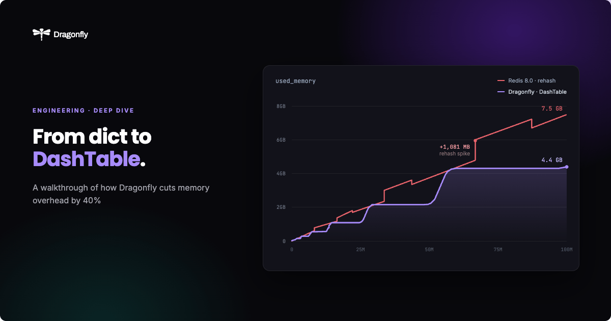
The theoretical numbers hold up under measurement. The chart below tracks used_memory reported by each server as 100 million keys are inserted into a fresh instance (pipeline=100), with both systems running on the same hardware under identical conditions (dragonfly with 1 proactor thread to match redis single threaded nature).

The vertical dashed lines mark the moments Redis allocates ht[1], initiating a rehash. Each line is annotated with the instantaneous memory spike: +41 MB at 2.2M keys, +73 MB at 4.3M, +142 MB at 8.4M, +273 MB at 16.8M, +542 MB at 33.6M, and +1,081 MB at 67.1M keys. These spikes are substantial. At 67 million keys, Redis temporarily allocates more than a gigabyte of additional memory solely for dictionary infrastructure, then gradually reclaims it as migration completes.

Dragonfly's curve is smooth by comparison. There are no visible jumps because segment splits redistribute at most 840 keys at a time, making each split effectively invisible at this scale. Memory growth remains nearly linear, with a slope that closely matches the approximately 18.7 bytes-per-entry cost derived in the earlier memory analysis.

At 100 million keys, Redis consumes roughly 7.5 GB of memory, while Dragonfly uses about 4.3 GB—a reduction of approximately 43%. This difference is consistent with the underlying data structures: Redis pays for dictEntry nodes and expanding bucket arrays, while Dragonfly's DashTable stores entries much more compactly.

The shape of the curves is as important as the final numbers. Redis exhibits a sawtooth pattern because memory consumption is discontinuous; operators must provision enough headroom to survive the next rehash spike or risk running out of memory during a resize. Dragonfly's gradual growth allows memory limits to be set much closer to actual data requirements, without reserving capacity for large, unpredictable rehash events.

Final Thought

Extendible hashing dates to 1979. Dragonfly's dashtable builds on a 2020 adaptation of it (Dash), reworking the idea into the backbone of a production in-memory store.

It's a good hash table.

[^1]: Redis has since responded to the rehash latency problem with `kvstore` (introduced in Redis 7.x) - but it's worth being precise about what that is, because the name invites confusion. `kvstore` is not cluster sharding. It has nothing to do with slots or separate instances. It is an array of ordinary `dict` structs living inside a single process, under a single database. When you `SET k v`, Redis hashes the key and picks which internal dict it lands in; from the outside it still looks like one database. The motivation is purely mechanical: one dict holding 100M keys has painful rehash events; eight dicts holding 12M keys each have rehash events that are 8x smaller and finish faster. It is the same trick Dragonfly uses with its per-thread shards - except Dragonfly's shards run on genuinely parallel threads and do real concurrent work. Redis's `kvstore` shards all run on the same event loop, so there is no parallelism gain, only smaller batches. Redis's answer to rehash latency was to chop one big dict into several smaller ones. DashTable's answer was to make the split itself O(1) by design, so the problem never accumulates in the first place. Same root problem, different levels of solution.